Integrals and the Fundamental Theorem of Calculus

(cod: P-67-38-6) The objective of this exercise is to explore the concept of definite integrals.

Consider a function \(f\) defined on an interval \([a,b]\). A partition of the interval \([a,b]\) is a division of \([a,b]\) into subintervals. More precisely, a partition is obtained by choosing points \[\small{a = x_0 < x_1 < x_2 < \cdots < x_{n-1} < x_n = b},\] such that the interval \([a,b]\) is divided into \(n\) subintervals \[ [x_0,x_1], [x_1,x_2], \dots, [x_{n-1},x_n]. \] In each subinterval of the partition, we choose a sample point. For \( i \in \{1,2,\dots,n\}\), we denote the \(i\)-th sample point by \[x_i^* \in [x_{i-1},x_i]\] and denote the length of the \(i\)-th subinterval by \[\Delta x_i = x_i - x_{i-1}\]. Given these choices, we then have a Riemann sum for \(f\) given by \[\small{f(x_1^*)\Delta x_1 + f(x_2^*)\Delta x_2 + \cdots + f(x_n^*) \Delta x_n},\] or, using sigma notation, \[\sum_{i=1}^n f(x_i^*) \Delta x_i.\] The figure below illustrates the situation with \(n = 6\). In it, the bases of the rectangles represent the subintervals of the partition (we do not display the points \(x_1, x_2, \dots, x_n\) of the partition, only the sample points).

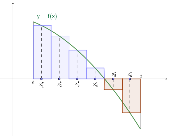
In the example above, each of the first four terms of the Riemann sum represents the area of a blue rectangle, while the last and penultimate terms are negative (since \(f\) is negative at the last two sample points), and the value of each of these terms is obtained by multiplying the area of a pink rectangle by \((-1)\).

We say that \(f\) is integrable on the interval \([a,b]\) if there exists a number \(L\) such that \[ \lim\limits_{\text{max } \Delta x_i \to 0} \sum_{i=1}^n f(x_i^*) \Delta x_i = L,\] where this limit means that we can make a Riemann sum as close as we want to \(L\), regardless of the choice of sample points, provided that the maximum length of the subintervals of the partition is sufficiently small. In this case, we say that the definite integral of \(f\) from \(a\) to \(b\) is equal to \(L\). We use the notation \(\int_a^b f(x) \, dx\) to represent this integral, so that \[\int_a^b f(x) \, dx = \lim\limits_{\text{max } \Delta x_i \to 0} \sum_{i=1}^n f(x_i^*) \Delta x_i.\]

There is an important theorem that guarantees that if \(f\) is continuous on \([a,b]\), then \(f\) is integrable on \([a,b]\).

Given \(f\) as a continuous function on \([a,b]\) (hence integrable), we can approximate the value of the integral of \(f\) by systematically taken Riemann sums. For each \(n \in \mathbb{N}\), let us take a regular partition of \([a,b]\) into \(n\) subintervals of equal length \(\Delta x = \dfrac{b-a}{n}\). Note that \(\Delta x \longrightarrow 0\) as \(n \longrightarrow + \infty\). Thus, regardless of the choice of sample points, we have that \[\int_a^b f(x) \, dx = \lim\limits_{n \to + \infty} \sum_{i=1}^n f(x_i^*) \Delta x.\] Of course, once a regular partition is fixed, there are numerous distinct ways to choose sample points. Some common choices include, for example, taking the midpoint of each subinterval as the sample point. In the animation below, which illustrates the process as \(n\) increases, we use the right endpoint of each subinterval as the sample point. For this choice, the associated Riemann sum is called the right Riemann sum.

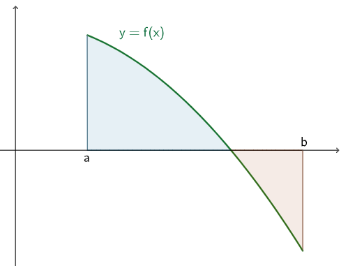
We observe that when the function \(f\) is non-negative on the interval \([a,b]\) (that is, \(f(x) \geq 0\) for all \(x \in [a,b]\)), the integral of \(f\) represents the area of the region between the x-axis and the graph of \(f\), with \(x\) between \(a\) and \(b\). However, this is not the case in general. In the example of our illustration, the value of the integral can be geometrically interpreted as the difference between the area of the blue region and the area of the pink region, as indicated below.

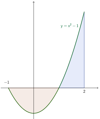
Let us now consider a specific example. Consider the function \(f(x) = x^2 - 1\) and the interval \([-1,2]\). For each \(n\), consider the right Riemann sum of \(f\) on this interval. We have that \[\Delta x = \dfrac{2 - (-1)}{n} = \dfrac{3}{n}\] and that the \(i\)-th sample point is given by \[x_i^* = x_{i+1} = -1 + i\left(\dfrac{3}{n}\right).\] Thus, we have that \[f(x_i^*) = \left(-1 + \dfrac{3i}{n}\right)^2 - 1 = \dfrac{9i^2}{n^2} - \dfrac{6i}{n}.\] Therefore, \[f(x_i^*)\Delta x = 9 \left(\dfrac{3i^2}{n^3} - \dfrac{2i}{n^2} \right).\] By working algebraically with the expression of the Riemann sum and then calculating the limit, we can conclude that

\begin{eqnarray*} \int_{-1}^2 (x^2 - 1) \, dx &=& \lim\limits_{n \to + \infty} 3 \left(\dfrac{n^2+1}{2n^2} \right) \\ & & \\ &=& 3/2. \end{eqnarray*}

\begin{eqnarray*} \int_{-1}^2 (x^2 - 1) \, dx &=& \lim\limits_{n \to + \infty} 9 \left(\dfrac{2n^2-1}{2n^2} \right) \\ & & \\ &=& 9. \end{eqnarray*}

\begin{eqnarray*} \int_{-1}^2 (x^2 - 1) \, dx &=& \lim\limits_{n \to + \infty} 3 \left(\dfrac{n^2-1}{2n^2} \right) \\ & & \\ &=& 0. \end{eqnarray*}

\begin{eqnarray*} \int_{-1}^2 (x^2 - 1) \, dx &=& \lim\limits_{n \to + \infty} 9 \left(\dfrac{n+1}{2n^2} \right) \\ & & \\ &=& 0. \end{eqnarray*}

\begin{eqnarray*} \int_{-1}^2 (x^2 - 1) \, dx &=& \lim\limits_{n \to + \infty} 3 \left(\dfrac{2n^2-1}{2n^2} \right) \\ & & \\ &=& 3. \end{eqnarray*}