Applications of Integration

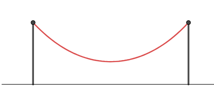
(cod: P-79-49-12) Consider a flexible and homogeneous cable suspended by its ends, attached to poles, both at the same height. The cable then assumes the shape of a curve known as a catenary (it is worth studying the history of this problem).

The objective of this exercise is to describe an expression for such a curve and study its properties.

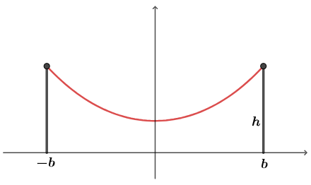
Assume that the height of the poles is \(h\) and the distance between the poles is \(2b\). We will position the \(x\) axis at ground level and the \(y\) axis as shown in the figure, assuming that the curve is the graph of a differentiable function \(y = f(x)\) that is even (symmetric with respect to the \(y\) axis).

Let \(P\) denote the lowest point of the curve, as shown in the figure below, and let \(Q = (x,f(x))\) be any point on the curve, with \(x>0\). We will describe the forces acting on the segment of the curve between points \(P\) and \(Q\).

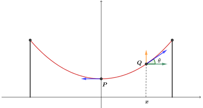
The tension force in the rope is tangent to the curve and can be decomposed into horizontal and vertical components (note that such force is horizontal at point \(P\)). Let \(T(x)\) denote the magnitude of the tension force at \(Q\). If \(\theta = \theta(x)\) is the angle described in the figure, then, since there is no motion, we must have \begin{equation}\label{comp1}T_0 = T(x) \cos(\theta(x)). \end{equation} Note, in particular, that the magnitude of the horizontal component of the tension, given by \(T(x) cos(\theta(x))\), is the same at any point (it does not depend on \(x\)).

From the vertical perspective, we have that \[p(x) = T(x) \sin(\theta(x)),\] where \(p(x)\) is the weight of the cable between \(P\) and \(Q\). Since the cable is homogeneous, let \(\rho\) denote the weight of the cable per unit length and \(L(x)\) the length of the segment of the curve between \(P\) and \(Q\). We then have that \[p(x) = \rho L(x),\] that is, \begin{equation}\label{comp2}\rho L(x) = T(x) \sin(\theta(x)). \end{equation} From (\ref{comp1}) and (\ref{comp2}), we conclude that \[f'(x) = \tan(\theta(x)) = \dfrac{\rho L(x)}{T_0}.\] Considering the constant \[a = \dfrac{\rho}{T_0},\] we have that \[f'(x) = a L(x),\] where the length \(L(x)\) is given by \[L(x) = \int_0^x \sqrt{1 + (f'(t))^2} \, dt.\] By the Fundamental Theorem of Calculus, \(L'(x) = \sqrt{1 + (f'(x))^2}\), thus \begin{eqnarray*} & & f''(x) = a \sqrt{1 + (f'(x))^2} \\ & & \\ &\iff& \dfrac{f''(x)}{\sqrt{1 + (f'(x))^2}} = a. \end{eqnarray*} We then want to obtain a function \(f(x)\) that satisfies the above equation (such an equation is called a second-order differential equation). Writing \(v(x) = f'(x)\), the above differential equation can be written more simply (becoming a first-order equation): \[\dfrac{v'(x)}{\sqrt{1 + (v(x))^2}} = a.\] This equation can be solved by integrating both sides. In the integral that arises on the left side, we can make the substitution \(u = v(x)\), obtaining \[\int\dfrac{1}{{\sqrt{1 + u^2}}} \, du,\] where we observe that the integrand is the derivative of the inverse hyperbolic sine. Therefore, we obtain \begin{eqnarray*} & & \operatorname{arsinh}\, (v(x)) = ax + B \\ & & \\ &\iff& v(x) = \sinh\, (ax+B) \\ & & \\ &\iff& f'(x) = \sinh\, (ax+B). \end{eqnarray*} Consider the following questions:

(i) Use \(f'(0)\) to define the value of the constant \(B\). Then, integrate again to obtain the expression for \(f(x)\). In doing so, a new integration constant will arise. Use the value of \(f(b)\) to determine this constant and define the expression for \(f(x)\).

(ii) Determine the length of this catenary. Knowing that the function is even, the length of the catenary will be twice the length of the segment in the first quadrant (segment with positive \(x\)).

(iii) The expression of the catenary depends on the parameter \(a\). To make this clear, let us denote the catenary by \(y = f_a(x)\) and its length by \(\mathcal{L}_a\). Determine the values of the limits \[\lim\limits_{a \to 0^+} f_a(0) \, \, \, \text{ and } \, \, \, \lim\limits_{a \to 0^+} \mathcal{L}_a.\]